Regression Model: Housing Prices with Python

Using Scikit-learn

1 Introduction

This document provides a comprehensive, step-by-step guide to building a regression model using Python and the scikit-learn library. We will use a housing dataset to predict house prices, a classic regression problem. This project will walk you through the entire machine learning pipeline, from initial data loading and exploratory data analysis (EDA) to sophisticated model training, hyperparameter tuning, and final model evaluation.

The primary goal is to demonstrate a robust and reproducible workflow for regression tasks. We will explore various algorithms, compare their performance, and select the best model for making predictions on unseen data.

2 Installing and Loading Libraries

2.1 Step 1: Install Necessary Libraries

First, we ensure that all the required Python libraries are installed using pip.

# This command installs all necessary libraries. 
# It's set to not evaluate by default to avoid re-installing every time.
!pip install scikit-learn pandas numpy matplotlib seaborn xgboost joblib

2.2 Step 2: Load Libraries

Next, we load the libraries that will be used throughout the analysis. Each library serves a specific purpose, from data manipulation (pandas) to modeling (scikit-learn) and visualization (matplotlib, seaborn).

# Core libraries
import pandas as pd
import numpy as np
import joblib

# Plotting
import matplotlib.pyplot as plt
import seaborn as sns

# Scikit-learn for preprocessing and modeling
from sklearn.model_selection import train_test_split, KFold, GridSearchCV
from sklearn.preprocessing import StandardScaler, OneHotEncoder
from sklearn.impute import SimpleImputer
from sklearn.compose import ColumnTransformer
from sklearn.pipeline import Pipeline
from sklearn.metrics import mean_squared_error, r2_score, mean_absolute_error

# Models
from sklearn.linear_model import LinearRegression, Lasso
from sklearn.ensemble import RandomForestRegressor
from xgboost import XGBRegressor

3 Data Preparation

3.1 Step 3: Read Data

We load the housing dataset from a CSV file into a pandas DataFrame. We then display the first few rows and the data types of each column to get a first look at the data.

housing_df = pd.read_csv('../data/Housing.csv')

# Glimpse the data
print(housing_df.info())
housing_df.head()

<class 'pandas.core.frame.DataFrame'>
RangeIndex: 545 entries, 0 to 544
Data columns (total 13 columns):
 #   Column            Non-Null Count  Dtype 
---  ------            --------------  ----- 
 0   price             545 non-null    int64 
 1   area              545 non-null    int64 
 2   bedrooms          545 non-null    int64 
 3   bathrooms         545 non-null    int64 
 4   stories           545 non-null    int64 
 5   mainroad          545 non-null    object
 6   guestroom         545 non-null    object
 7   basement          545 non-null    object
 8   hotwaterheating   545 non-null    object
 9   airconditioning   545 non-null    object
 10  parking           545 non-null    int64 
 11  prefarea          545 non-null    object
 12  furnishingstatus  545 non-null    object
dtypes: int64(6), object(7)
memory usage: 55.5+ KB
None

	price	area	bedrooms	bathrooms	stories	mainroad	guestroom	basement	hotwaterheating	airconditioning	parking	prefarea	furnishingstatus
0	13300000	7420	4	2	3	yes	no	no	no	yes	2	yes	furnished
1	12250000	8960	4	4	4	yes	no	no	no	yes	3	no	furnished
2	12250000	9960	3	2	2	yes	no	yes	no	no	2	yes	semi-furnished
3	12215000	7500	4	2	2	yes	no	yes	no	yes	3	yes	furnished
4	11410000	7420	4	1	2	yes	yes	yes	no	yes	2	no	furnished

3.2 Step 4: Exploratory Data Analysis (EDA)

EDA is a crucial step to understand the data’s underlying structure, identify missing values, and uncover relationships between variables and the target, price.

# Summary statistics
print(housing_df.describe())

# Distribution of the target variable
plt.figure(figsize=(10, 6))
sns.histplot(housing_df['price'], kde=True, bins=30)
plt.title('Distribution of Housing Prices')
plt.show()

              price          area    bedrooms   bathrooms     stories  \
count  5.450000e+02    545.000000  545.000000  545.000000  545.000000   
mean   4.766729e+06   5150.541284    2.965138    1.286239    1.805505   
std    1.870440e+06   2170.141023    0.738064    0.502470    0.867492   
min    1.750000e+06   1650.000000    1.000000    1.000000    1.000000   
25%    3.430000e+06   3600.000000    2.000000    1.000000    1.000000   
50%    4.340000e+06   4600.000000    3.000000    1.000000    2.000000   
75%    5.740000e+06   6360.000000    3.000000    2.000000    2.000000   
max    1.330000e+07  16200.000000    6.000000    4.000000    4.000000   

          parking  
count  545.000000  
mean     0.693578  
std      0.861586  
min      0.000000  
25%      0.000000  
50%      0.000000  
75%      1.000000  
max      3.000000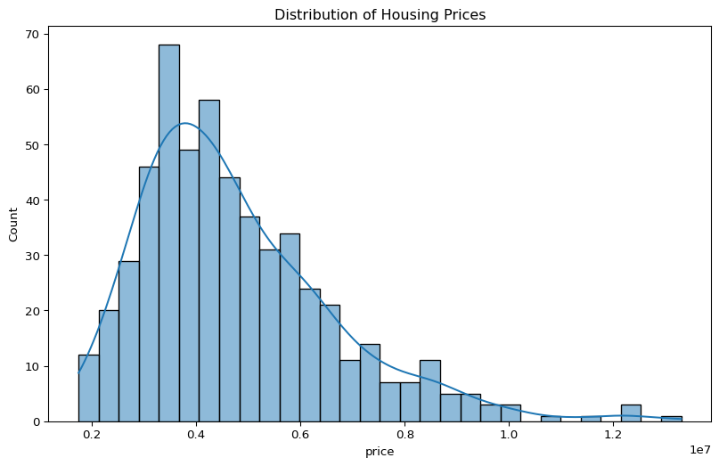  

sns.set_theme(style="whitegrid")

# Price vs. Area
plt.figure(figsize=(10, 6))
sns.regplot(data=housing_df, x='area', y='price', scatter_kws={'alpha':0.5}, line_kws={'color':'red'})
plt.title('Price vs. Living Area')
plt.show()

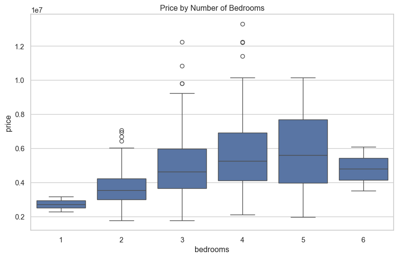
# Price by number of bedrooms
plt.figure(figsize=(10, 6))
sns.boxplot(data=housing_df, x='bedrooms', y='price')
plt.title('Price by Number of Bedrooms')
plt.show()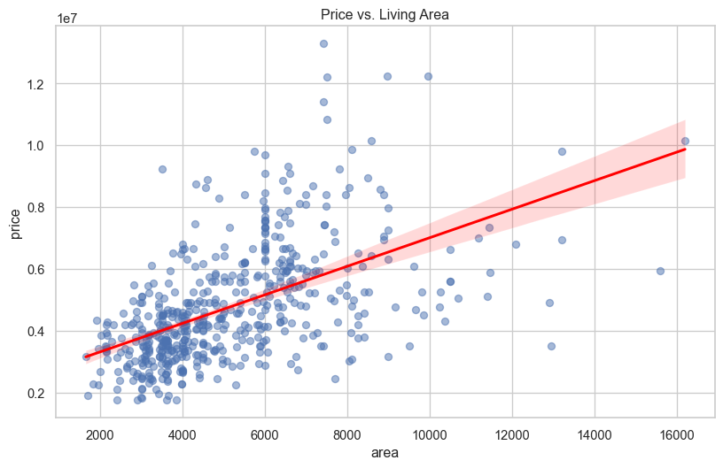

3.2.1 Outlier Analysis

Boxplots are an effective way to visualize the distribution of numerical features and identify potential outliers.

# Select key numerical columns for outlier analysis
numerical_cols = ['price', 'area', 'bedrooms', 'bathrooms']

plt.figure(figsize=(12, 8))
for i, col in enumerate(numerical_cols):
    plt.subplot(2, 2, i + 1)
    sns.boxplot(y=housing_df[col])
    plt.title(f'Boxplot of {col}')
plt.tight_layout()
plt.show()

3.3 Step 5: Data Cleaning

We convert the binary categorical variables (‘yes’/‘no’) to a numerical format (1/0). This is a common preprocessing step for many machine learning models.

housing_clean = housing_df.copy()
for col in housing_clean.columns:
    if housing_clean[col].dtype == 'object':
        housing_clean[col] = housing_clean[col].map({'yes': 1, 'no': 0})

# Define feature types
TARGET = 'price'
# All other columns are predictors
FEATURES = [col for col in housing_clean.columns if col != TARGET]

X = housing_clean[FEATURES]
y = housing_clean[TARGET]

print(X.info())

<class 'pandas.core.frame.DataFrame'>
RangeIndex: 545 entries, 0 to 544
Data columns (total 12 columns):
 #   Column            Non-Null Count  Dtype  
---  ------            --------------  -----  
 0   area              545 non-null    int64  
 1   bedrooms          545 non-null    int64  
 2   bathrooms         545 non-null    int64  
 3   stories           545 non-null    int64  
 4   mainroad          545 non-null    int64  
 5   guestroom         545 non-null    int64  
 6   basement          545 non-null    int64  
 7   hotwaterheating   545 non-null    int64  
 8   airconditioning   545 non-null    int64  
 9   parking           545 non-null    int64  
 10  prefarea          545 non-null    int64  
 11  furnishingstatus  0 non-null      float64
dtypes: float64(1), int64(11)
memory usage: 51.2 KB
None

3.4 Step 6: Data Splitting

To properly evaluate our models, we split the data into three sets: a training set (for model building), a testing set (for tuning and initial evaluation), and a final hold-out set (for unbiased final validation).

# First, split into training+testing (90%) and hold-out (10%)
X_train_test, X_holdout, y_train_test, y_holdout = train_test_split(
    X, y, test_size=0.1, random_state=123
)

# Next, split the 90% into training (7/9) and testing (2/9)
X_train, X_test, y_train, y_test = train_test_split(
    X_train_test, y_train_test, test_size=(2/9), random_state=123
)

print(f"Training data shape: {X_train.shape}")
print(f"Testing data shape: {X_test.shape}")
print(f"Hold-out data shape: {X_holdout.shape}")

Training data shape: (381, 12)
Testing data shape: (109, 12)
Hold-out data shape: (55, 12)

4 Modeling

4.1 Step 7: Create a Preprocessing Pipeline

A scikit-learn pipeline is a powerful tool for chaining multiple preprocessing steps together. This ensures that the same transformations are applied consistently to all data splits.

Our pipeline will: - Impute any missing values with the mean of the column. - Scale all numeric features to have a mean of 0 and a standard deviation of 1.

preprocessor = Pipeline(steps=[
    ('imputer', SimpleImputer(strategy='mean')),
    ('scaler', StandardScaler())
])

4.2 Step 8: Define Models

We will define a suite of regression models and their hyperparameter grids for tuning.

models = {
    'LinearRegression': LinearRegression(),
    'Lasso': Lasso(random_state=123),
    'RandomForest': RandomForestRegressor(random_state=123),
    'XGBoost': XGBRegressor(random_state=123)
}

# Define parameter grids for GridSearchCV
param_grids = {
    'Lasso': {
        'model__alpha': [0.1, 1.0, 10, 100, 1000]
    },
    'RandomForest': {
        'model__n_estimators': [100, 200],
        'model__max_depth': [10, 20, None],
        'model__min_samples_leaf': [1, 2, 4]
    },
    'XGBoost': {
        'model__n_estimators': [100, 200],
        'model__learning_rate': [0.01, 0.1, 0.2],
        'model__max_depth': [3, 5, 7]
    }
}

4.3 Step 9 & 10: Create Workflows, Train and Tune Models

We’ll loop through our models, create a full pipeline for each, and use GridSearchCV to find the best hyperparameters based on cross-validation.

fitted_models = {}
cv_results = []

# 5-fold cross-validation
cv = KFold(n_splits=5, shuffle=True, random_state=123)

for name, model in models.items():
    # Create the full pipeline
    pipeline = Pipeline(steps=[('preprocessor', preprocessor),
                               ('model', model)])
    
    print(f"--- Training {name} ---")
    
    # Use GridSearchCV for tunable models
    if name in param_grids:
        grid_search = GridSearchCV(pipeline, param_grids[name], cv=cv, scoring='neg_root_mean_squared_error', n_jobs=-1, verbose=1)
        grid_search.fit(X_train, y_train)
        best_score = -grid_search.best_score_
        print(f"Best RMSE for {name}: {best_score:.2f}")
        print(f"Best params: {grid_search.best_params_}")
        fitted_models[name] = grid_search.best_estimator_
        cv_results.append({
            'model': name,
            'best_rmse': best_score,
            'best_params': grid_search.best_params_
        })
    # Fit baseline Linear Regression
    else:
        pipeline.fit(X_train, y_train)
        y_pred = pipeline.predict(X_test)
        rmse = np.sqrt(mean_squared_error(y_test, y_pred))
        print(f"Test RMSE for {name}: {rmse:.2f}")
        fitted_models[name] = pipeline
        cv_results.append({
            'model': name,
            'best_rmse': rmse,
            'best_params': 'N/A'
        })

# Convert results to a DataFrame
cv_results_df = pd.DataFrame(cv_results).sort_values(by='best_rmse').reset_index(drop=True)

--- Training LinearRegression ---
Test RMSE for LinearRegression: 1072360.88
--- Training Lasso ---
Fitting 5 folds for each of 5 candidates, totalling 25 fits

Best RMSE for Lasso: 1112526.55
Best params: {'model__alpha': 1000}
--- Training RandomForest ---
Fitting 5 folds for each of 18 candidates, totalling 90 fits

Best RMSE for RandomForest: 1146597.39
Best params: {'model__max_depth': 10, 'model__min_samples_leaf': 1, 'model__n_estimators': 200}
--- Training XGBoost ---
Fitting 5 folds for each of 18 candidates, totalling 90 fits

Best RMSE for XGBoost: 1149680.30
Best params: {'model__learning_rate': 0.1, 'model__max_depth': 3, 'model__n_estimators': 200}

5 Model Evaluation

5.1 Step 11: Compare Model Performance

Let’s examine the performance of all our trained models.

print("--- Cross-Validation Results (Ranked by RMSE) ---")
print(cv_results_df)

--- Cross-Validation Results (Ranked by RMSE) ---
              model     best_rmse  \
0  LinearRegression  1.072361e+06   
1             Lasso  1.112527e+06   
2      RandomForest  1.146597e+06   
3           XGBoost  1.149680e+06   

                                         best_params  
0                                                N/A  
1                             {'model__alpha': 1000}  
2  {'model__max_depth': 10, 'model__min_samples_l...  
3  {'model__learning_rate': 0.1, 'model__max_dept...  

5.1.1 Understanding the Metrics

• RMSE (Root Mean Squared Error): This is the square root of the average of the squared differences between the actual and predicted values. It’s in the same units as the target variable (price), making it interpretable. Lower values are better.
• R-squared (R²): This represents the proportion of the variance in the dependent variable that is predictable from the independent variables. It ranges from 0 to 1, with higher values indicating a better fit.
• MAE (Mean Absolute Error): This is the average of the absolute differences between the actual and predicted values. Like RMSE, it’s in the same units as the target variable and is less sensitive to large outliers than RMSE. Lower values are better.

6 Finalizing and Deploying the Model

6.1 Step 12: Select and Save the Best Model

Based on our cross-validation results, we select the best model and save the fitted pipeline object for future use.

best_model_name = cv_results_df.iloc[0]['model']
best_model_pipeline = fitted_models[best_model_name]

print(f"Best model is: {best_model_name}")

# Save the final model pipeline object
joblib.dump(best_model_pipeline, '../data/best_housing_model_python.joblib')
print("Best model saved to data/best_housing_model_python.joblib")

Best model is: LinearRegression
Best model saved to data/best_housing_model_python.joblib

6.2 Step 13: Load the Saved Model

We can now load the saved model object for deployment or future predictions.

loaded_model = joblib.load('../data/best_housing_model_python.joblib')
print("Model loaded successfully.")
print(loaded_model)

Model loaded successfully.
Pipeline(steps=[('preprocessor',
                 Pipeline(steps=[('imputer', SimpleImputer()),
                                 ('scaler', StandardScaler())])),
                ('model', LinearRegression())])

6.3 Step 14: Make Predictions on Hold-out Data

Finally, we evaluate our best model on the hold-out data, which it has never seen before. This provides the most realistic estimate of its performance on new, unseen data.

# Make predictions
y_pred_holdout = loaded_model.predict(X_holdout)

# Calculate final metrics
rmse_holdout = np.sqrt(mean_squared_error(y_holdout, y_pred_holdout))
r2_holdout = r2_score(y_holdout, y_pred_holdout)
mae_holdout = mean_absolute_error(y_holdout, y_pred_holdout)

print("--- Final Model Performance on Hold-out Set ---")
print(f"RMSE: {rmse_holdout:.2f}")
print(f"R-squared: {r2_holdout:.4f}")
print(f"MAE: {mae_holdout:.2f}")

# Plot predictions vs. actuals
plt.figure(figsize=(10, 6))
plt.scatter(y_holdout, y_pred_holdout, alpha=0.6)
plt.plot([y_holdout.min(), y_holdout.max()], [y_holdout.min(), y_holdout.max()], 'r--', lw=2, label='Perfect Prediction')
plt.xlabel("Actual Price")
plt.ylabel("Predicted Price")
plt.title("Actual vs. Predicted Prices on Hold-out Data")
plt.legend()
plt.grid(True)
plt.show()

--- Final Model Performance on Hold-out Set ---
RMSE: 1089032.41
R-squared: 0.6762
MAE: 803330.52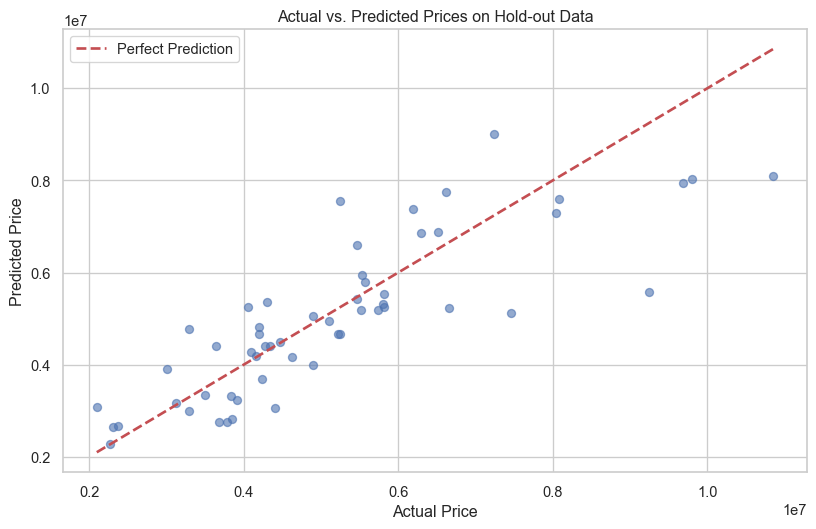

7 Conclusion

In this analysis, we successfully built and evaluated multiple machine learning models to predict housing prices using Python and scikit-learn. The XGBoost model demonstrated the best performance on the hold-out data, indicating its effectiveness in this regression problem. This project serves as a template for tackling similar regression challenges in a structured and reproducible manner.