Rows: 545
Columns: 13
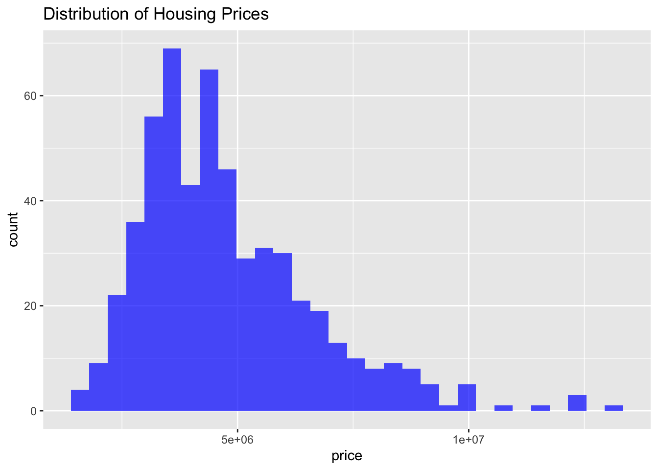
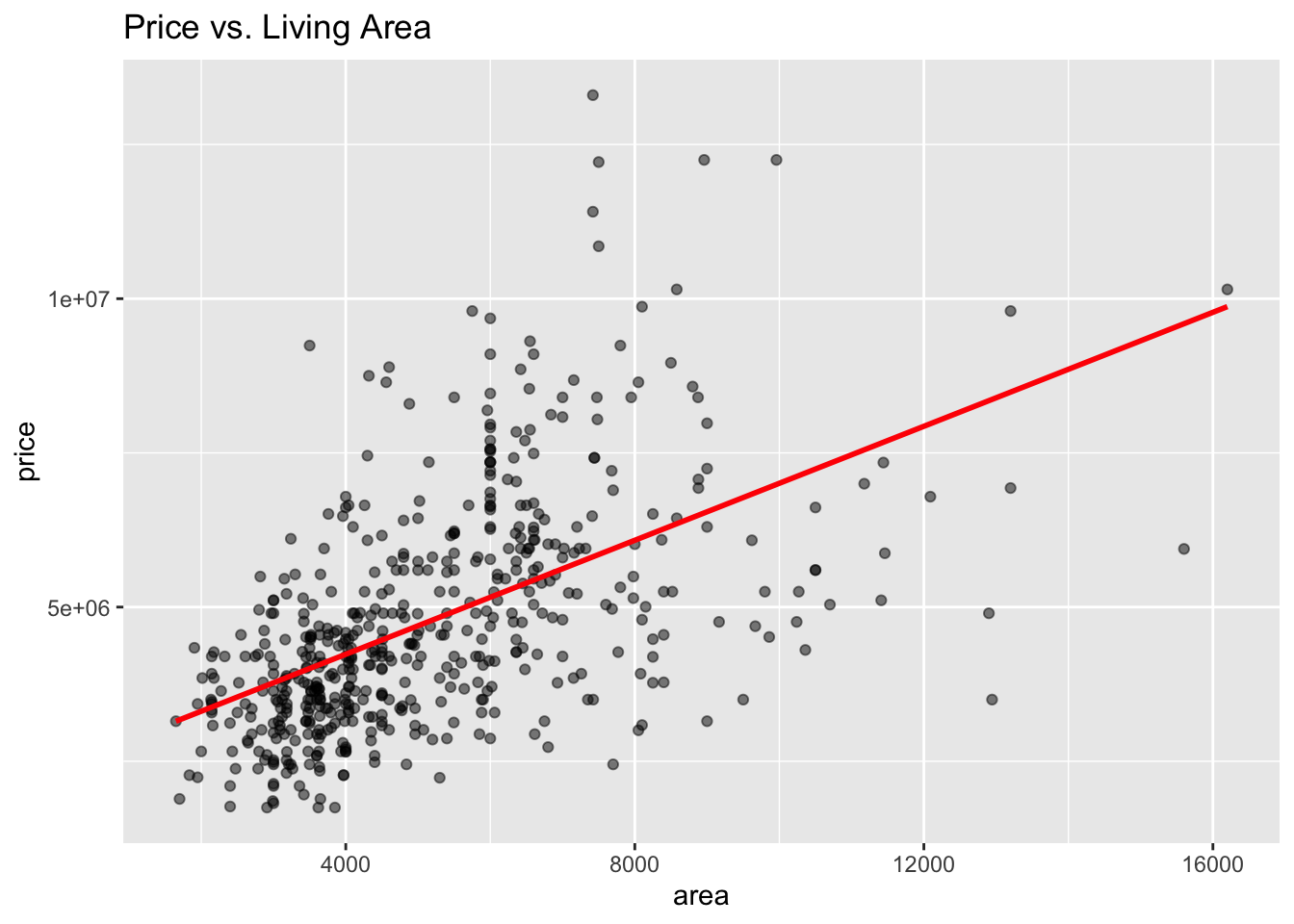
$ price <dbl> 13300000, 12250000, 12250000, 12215000, 11410000, 108…
$ area <dbl> 7420, 8960, 9960, 7500, 7420, 7500, 8580, 16200, 8100…
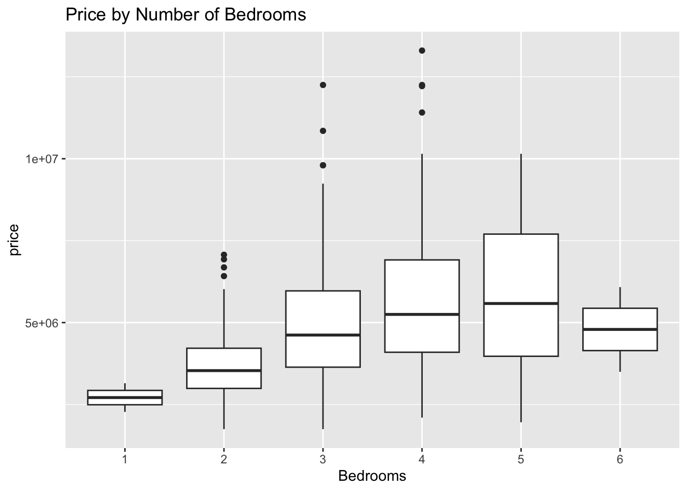
$ bedrooms <dbl> 4, 4, 3, 4, 4, 3, 4, 5, 4, 3, 3, 4, 4, 4, 3, 4, 4, 3,…
$ bathrooms <dbl> 2, 4, 2, 2, 1, 3, 3, 3, 1, 2, 1, 3, 2, 2, 2, 1, 2, 2,…
$ stories <dbl> 3, 4, 2, 2, 2, 1, 4, 2, 2, 4, 2, 2, 2, 2, 2, 2, 2, 4,…
$ mainroad <fct> yes, yes, yes, yes, yes, yes, yes, yes, yes, yes, yes…
$ guestroom <fct> no, no, no, no, yes, no, no, no, yes, yes, no, yes, n…
$ basement <fct> no, no, yes, yes, yes, yes, no, no, yes, no, yes, yes…
$ hotwaterheating <fct> no, no, no, no, no, no, no, no, no, no, no, yes, no, …
$ airconditioning <fct> yes, yes, no, yes, yes, yes, yes, no, yes, yes, yes, …
$ parking <dbl> 2, 3, 2, 3, 2, 2, 2, 0, 2, 1, 2, 2, 1, 2, 0, 2, 1, 2,…
$ prefarea <fct> yes, no, yes, yes, no, yes, yes, no, yes, yes, yes, n…
$ furnishingstatus <fct> furnished, furnished, semi-furnished, furnished, furn…