Code
library(tidyverse)This document provides a detailed overview of the fundamental data structures in R, with explanations and code examples.
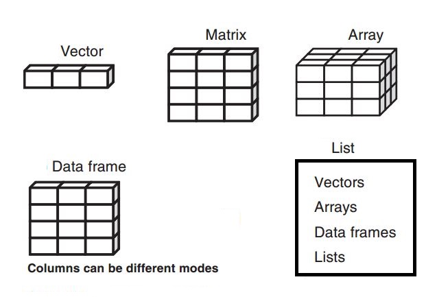
library(tidyverse)A vector is a one-dimensional, ordered collection of elements. A key characteristic of vectors is that all elements must be of the same data type (homogeneous). They are the simplest and most common data structure in R.
Here, we create a numeric vector using the c() (combine) function.
a = c(1, 2, 3, 4)
a
[1] 1 2 3 4The class() function confirms that the vector is of type “numeric”.
class(a)[1] "numeric"This example creates a character vector.
b =  c("Debi", "Sandeep", "Subham", "Shiba")
b
[1] "Debi" "Sandeep" "Subham" "Shiba" class(b)[1] "character"The seq() function generates a sequence of numbers.
seq(from = 2, to = 14, by = 2) [1] 2 4 6 8 10 12 14The rep() function repeats a value a specified number of times.
rep(x = 1.5, times = 4) [1] 1.5 1.5 1.5 1.5The sample() function takes a random sample from a set of elements. replace = FALSE means each element can only be chosen once.
sample(1:10, 5, replace = FALSE) [1] 9 2 7 4 8With replace = TRUE, elements can be chosen multiple times.
sample(1:10, 5, replace = TRUE) [1] 5 6 9 9 7runif() generates random numbers from a uniform distribution.
runif(1, min = 0, max = 1)[1] 0.6721013rnorm() generates random numbers from a normal distribution.
sn1 <- rnorm(4, mean = 0, sd = 1) # Standard normal distribution
sn1
[1] -0.9667081 0.3027156 0.7218398 -0.7725936The unique() function removes duplicate elements from a vector.
v1 = c(1, 1, 2, 2, 5, 6)
v1
[1] 1 1 2 2 5 6unique(v1)[1] 1 2 5 6You can combine vectors by using the c() function.
x = c(1, 2, 3)
y = c(4, 5, 6)
z = c(x, y)
z
[1] 1 2 3 4 5 6Negative indexing removes elements at the specified positions.
x = c(1, 2, 3, 4, 5)
x
[1] 1 2 3 4 5Remove the first element:
x[-1][1] 2 3 4 5Remove the last element:
x[-length(x)][1] 1 2 3 4Remove elements based on a vector of indices:
remove = c(2, 4)
x[-remove]
[1] 1 3 5sort() arranges vector elements in ascending or descending order.
a = c(2, 4, 6, 1, 4)
sort(a)
[1] 1 2 4 4 6sort(a, decreasing = TRUE)[1] 6 4 4 2 1length() returns the number of elements in a vector.
length(a)[1] 5Mathematical functions can be applied to entire vectors.
x = c(1, 2, 3, 4, 5)
sum(x)
[1] 15x = c(1, 2, 3, 6, 9, 10)Select the first element:
x[1][1] 1Select the last element:
x[length(x)][1] 10Select a range of elements:
x[1:3][1] 1 2 3setdiff(x, y) finds elements that are in vector x but not in vector y.
xx = c(1, 2, 3, 4)
yy = c(2, 4)
setdiff(xx, yy)
[1] 1 3as.* functions are used to coerce vectors from one type to another.
x <- c("a", "g", "b")
y = as.factor(x)
y
[1] a g b
Levels: a b gx <- c('123', '44', '222')
y = as.numeric(x)
y[1] 123 44 222A data frame is a two-dimensional, heterogeneous data structure, similar to a spreadsheet or a SQL table. Each column can have a different data type, but all elements within a column must be of the same type. It is the most common data structure for storing datasets in R.
Name = c("Amiya", "Raj", "Asish")
Language = c("R", "Python", "Java")
Age = c(22, 25, 45)

df = data.frame(Name, Language, Age)
df
Name Language Age
1 Amiya R 22
2 Raj Python 25
3 Asish Java 45Converting a data frame to a matrix will coerce all elements to the most flexible data type (usually character).
mat <- as.matrix(df)
mat
Name Language Age
[1,] "Amiya" "R" "22"
[2,] "Raj" "Python" "25"
[3,] "Asish" "Java" "45"You can extract a single column as a vector using $ or [[ ]] notation.
vec = df[['Name']]
vec
[1] "Amiya" "Raj" "Asish"A matrix is a two-dimensional, homogeneous data structure. All elements must be of the same type. It has a fixed number of rows and columns.
A = matrix(
    c(1, 2, 3, 4, 5, 6, 7, 8, 9),
    nrow = 3,
    ncol = 3,
    byrow = TRUE # Fill the matrix row by row
)
A
[,1] [,2] [,3]
[1,] 1 2 3
[2,] 4 5 6
[3,] 7 8 9Access the element in the 2nd row, 3rd column:
A [2, 3][1] 6Access the entire 1st row:
A[1, ][1] 1 2 3Access the entire 3rd column:
A [, 3][1] 3 6 9Matrices support element-wise mathematical operations.
matrix002 = A + A
matrix002
[,1] [,2] [,3]
[1,] 2 4 6
[2,] 8 10 12
[3,] 14 16 18A list is a one-dimensional, heterogeneous data structure. Unlike vectors, lists can contain elements of different types, including other lists, vectors, or even functions.
empId = c(1, 2, 3, 4)
empName = c("Debi", "Sandeep", "Subham", "Shiba")
numberOfEmp = 4

empList = list(ID = empId, Names = empName, Total = numberOfEmp)
empList
$ID
[1] 1 2 3 4
$Names
[1] "Debi" "Sandeep" "Subham" "Shiba"
$Total
[1] 4Use [[index]] or [[name]] to access the content of a single list element. Use $ as a shortcut for named elements.
Access the second element (a vector):
empList[[2]][1] "Debi" "Sandeep" "Subham" "Shiba" Access the element named “item3” (a data frame):
empList[["Names"]][1] "Debi" "Sandeep" "Subham" "Shiba" Use the $ operator for the same result:
empList$Names[1] "Debi" "Sandeep" "Subham" "Shiba" An array is a multi-dimensional, homogeneous data structure. It can have two or more dimensions.
This example creates a 3D array with 2 rows, 2 columns, and 2 “layers”.
my_array = array(
    c(1, 2, 3, 4, 5, 6, 7, 8),
    dim = c(2, 2, 2)
)
my_array
, , 1
     [,1] [,2]
[1,]    1    3
[2,]    2    4
, , 2
[,1] [,2]
[1,] 5 7
[2,] 6 8Elements are accessed using [row, column, dimension] notation.
Access the element in the 1st row, 2nd column of the 2nd dimension (layer):
my_array[1, 2, 2][1] 7Access the entire first matrix (1st layer):
my_array[, , 1] [,1] [,2]
[1,] 1 3
[2,] 2 4Understanding the structure of your data is a critical first step in any analysis. R provides several useful functions for this.
The str() (structure) function is one of the most useful diagnostic tools in R. It provides a compact, human-readable summary of any R object, showing its type, dimensions, and a preview of its content.
str(df)'data.frame': 3 obs. of 3 variables:
$ Name : chr "Amiya" "Raj" "Asish"
$ Language: chr "R" "Python" "Java"
$ Age : num 22 25 45str(empList)List of 3
$ ID : num [1:4] 1 2 3 4
$ Names: chr [1:4] "Debi" "Sandeep" "Subham" "Shiba"
$ Total: num 4class(): Returns the high-level class of an object.typeof(): Returns the internal storage type of an object.length(): Returns the number of elements in a vector or list.dim(): Returns the dimensions (e.g., rows and columns) of a data frame, matrix, or array.names() or colnames(): Returns the column names of a data frame, matrix, or list.# Create a sample data frame
inspect_df <- data.frame(
ID = 1:3,
Product = c("A", "B", "C"),
Price = c(10.5, 20.0, 15.2)
)
class(inspect_df)[1] "data.frame"dim(inspect_df)[1] 3 3names(inspect_df)[1] "ID" "Product" "Price" https://www.geeksforgeeks.org/data-structures-in-r-programming/