Code
library(reticulate)
py_require(c('celluloid','seaborn','IPython'))![]()
library(reticulate)
py_require(c('celluloid','seaborn','IPython'))Seaborn is a Python data visualization library based on Matplotlib. It provides a high-level interface for creating attractive and informative statistical graphics. This document demonstrates how to create various plots using Seaborn, customize their appearance, and save them.
import seaborn as sns
print(sns.__version__)0.13.2# Import necessary libraries
import seaborn as sns
import pandas as pd
import matplotlib.pyplot as plt
import matplotlib
# Load an example dataset
tips = sns.load_dataset("tips")
tips.head() total_bill tip sex smoker day time size
0 16.99 1.01 Female No Sun Dinner 2
1 10.34 1.66 Male No Sun Dinner 3
2 21.01 3.50 Male No Sun Dinner 3
3 23.68 3.31 Male No Sun Dinner 2
4 24.59 3.61 Female No Sun Dinner 4A scatter plot is used to display the relationship between two continuous variables. Each point on the plot represents an observation in the dataset.
sns.scatterplot(data=tips, x='tip', y='total_bill')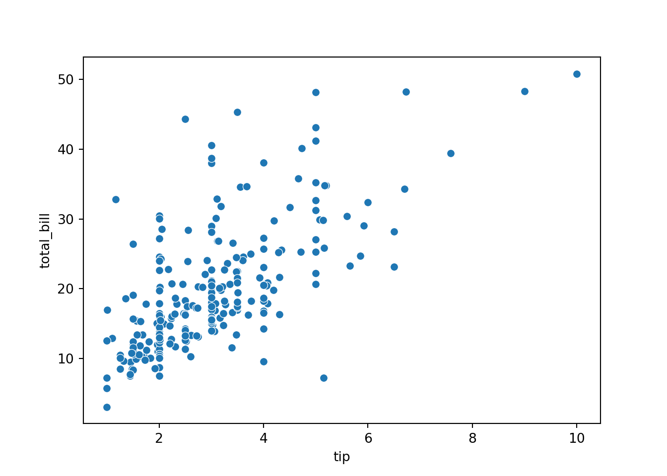
You can color the points in a scatter plot based on a categorical variable to visualize relationships within different groups.
sns.scatterplot(data=tips, x='tip', y='total_bill', hue='sex')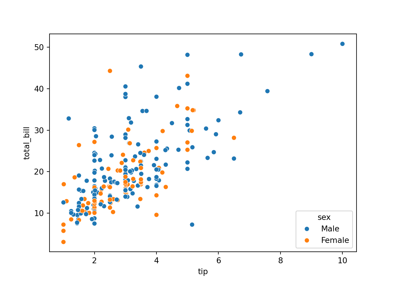
Similarly, the size of the points can be varied based on a numerical or categorical variable.
sns.scatterplot(data=tips, x='tip', y='total_bill', size='size')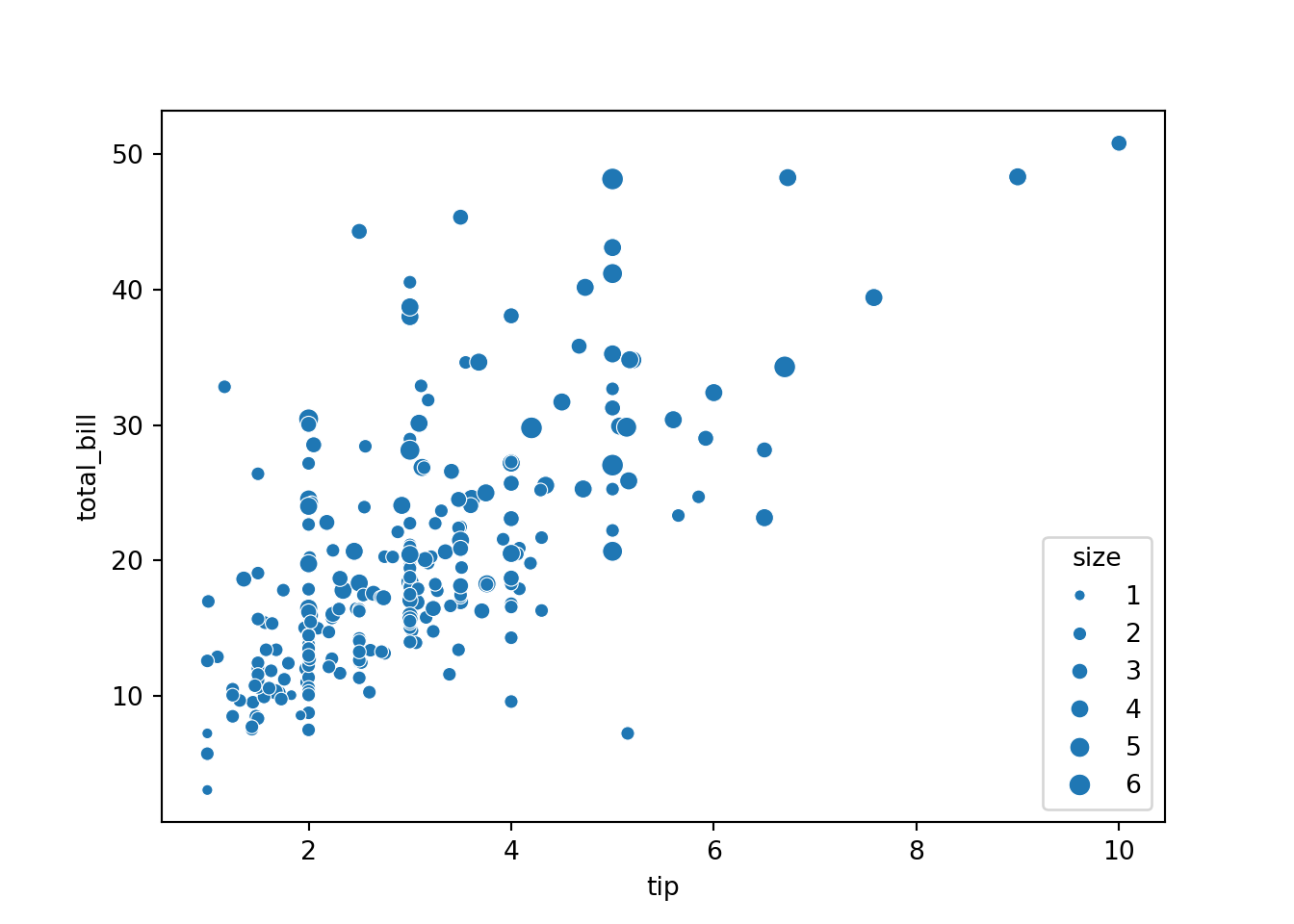
A line plot is ideal for visualizing the trend of a continuous variable over a continuous interval or time.
dowjones = sns.load_dataset("dowjones")
dowjones.head()
Date Price
0 1914-12-01 55.00
1 1915-01-01 56.55
2 1915-02-01 56.00
3 1915-03-01 58.30
4 1915-04-01 66.45sns.lineplot(data=dowjones, x='Date', y='Price')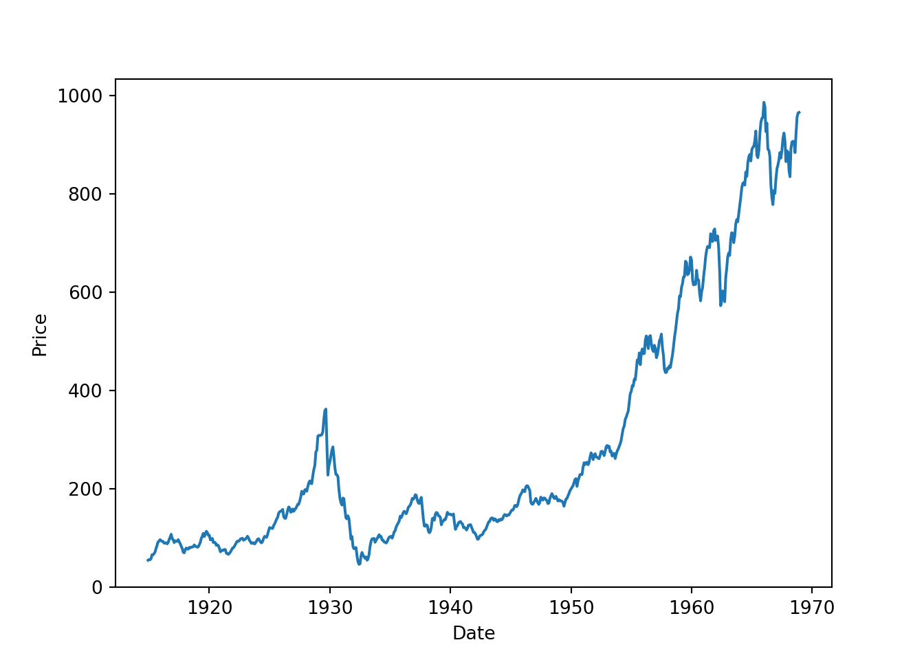
You can also add markers to the line plot to highlight the data points. ::: {.cell}
sns.lineplot(data=dowjones, x='Date', y='Price', marker='o')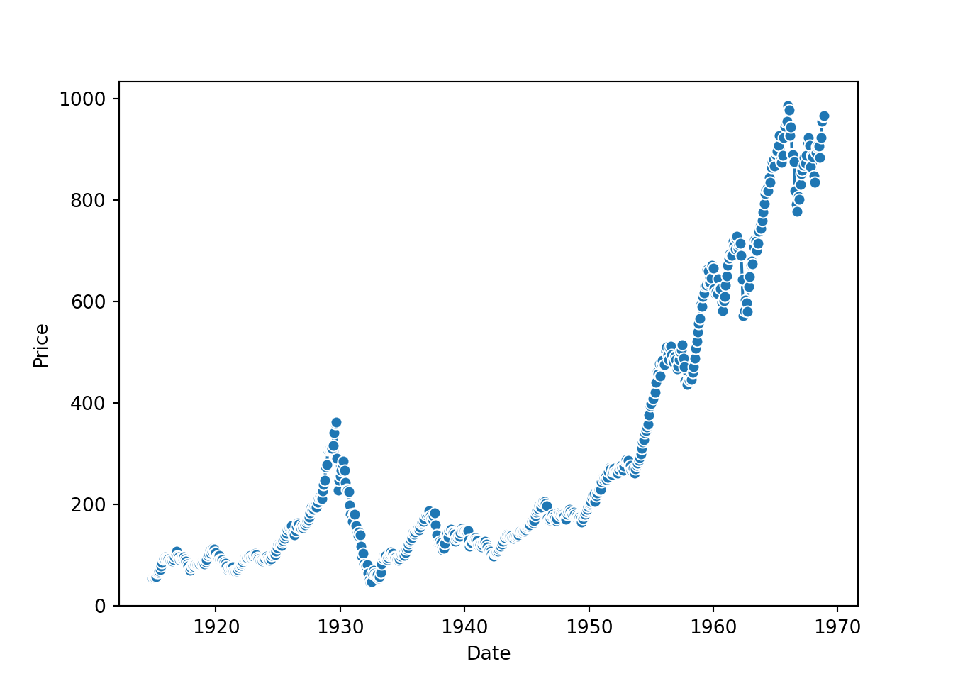
:::
Different lines can be plotted for different categories to compare trends.
import random

# Create datasets for comparison
dowjones2 = dowjones.copy()
dowjones2['type'] = 'old'

dowjones3 = dowjones.copy()
dowjones3['Price'] = dowjones3['Price'] + random.random() * 200
dowjones3['type'] = 'new'

dowjones4 = pd.concat([dowjones2, dowjones3], ignore_index=True)
dowjones4 = dowjones4.sort_values('Date').reset_index(drop=True)dowjones4.head() Date Price type
0 1914-12-01 55.000000 old
1 1914-12-01 148.624455 new
2 1915-01-01 150.174455 new
3 1915-01-01 56.550000 old
4 1915-02-01 56.000000 oldsns.lineplot(data=dowjones4, x='Date', y='Price', hue='type')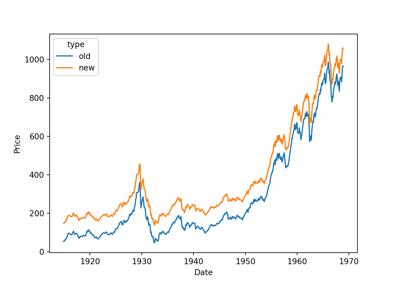
A histogram is used to represent the distribution of a single numerical variable.
sns.histplot(data=tips, x='tip')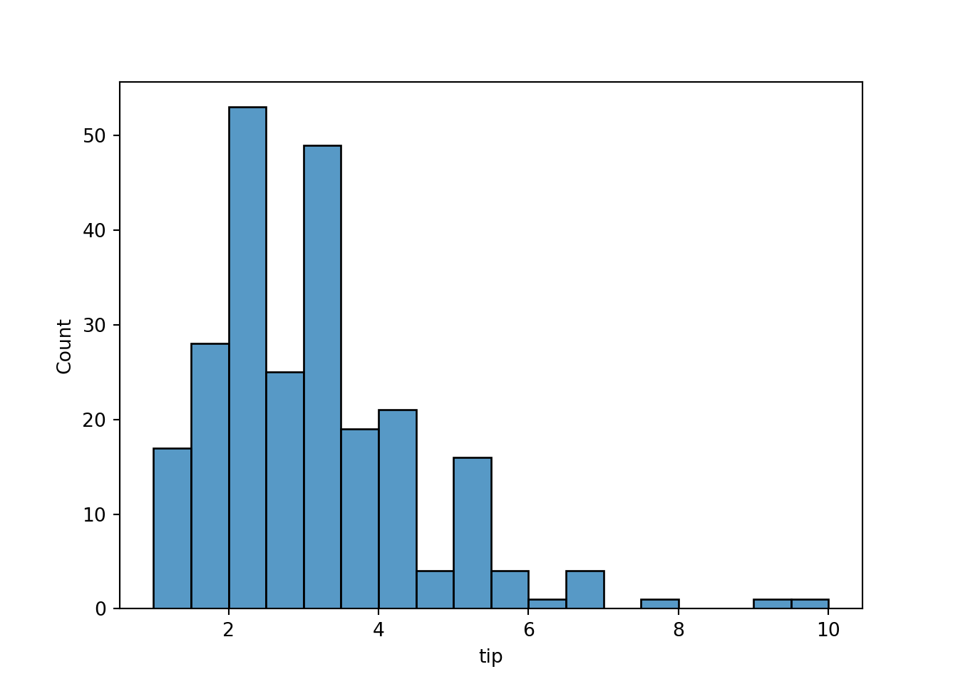
Histograms can be grouped by a categorical variable to compare distributions.
sns.histplot(data=tips, x='tip', hue='sex', multiple="dodge")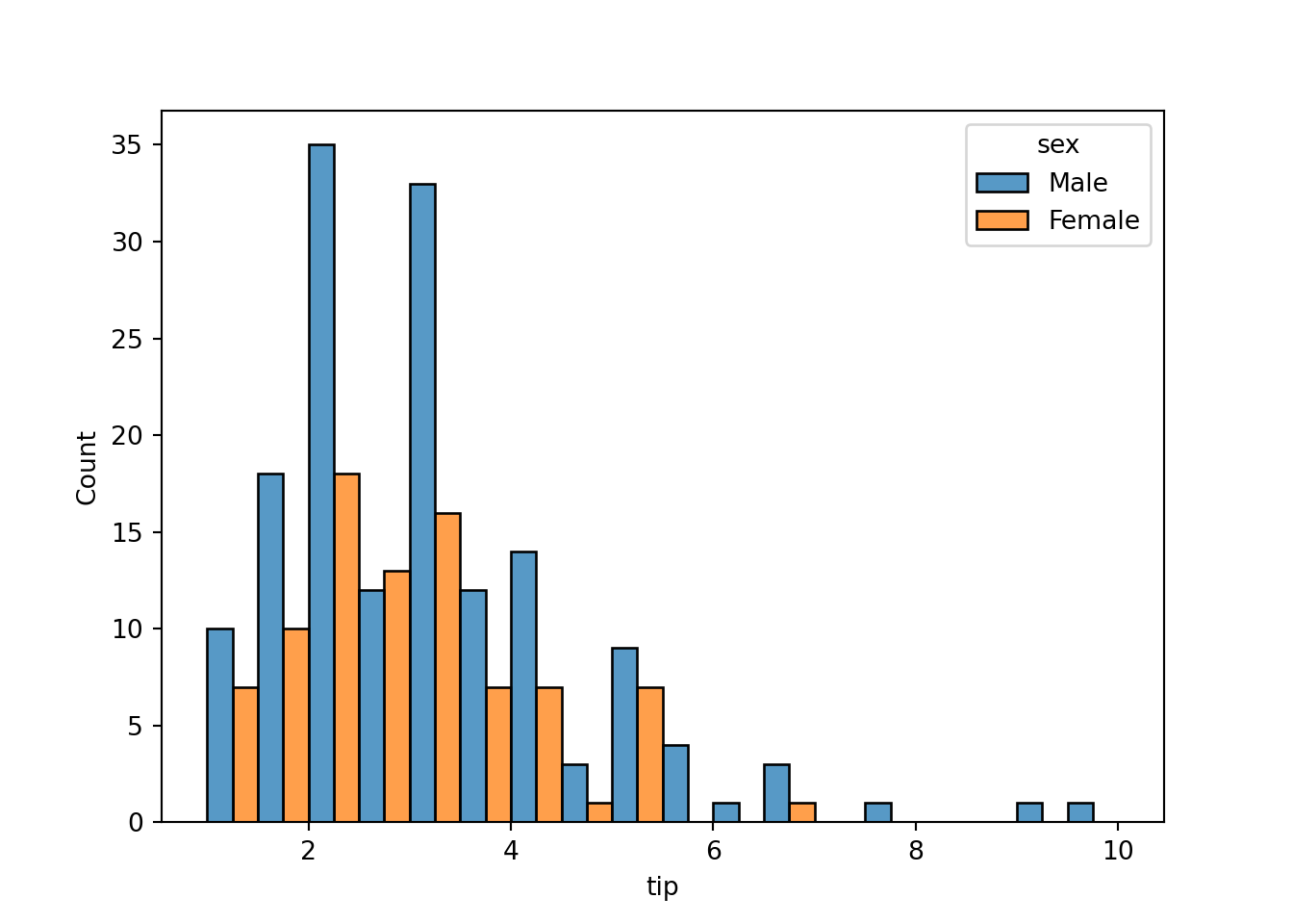
A bar chart represents categorical data with rectangular bars. The lengths of the bars are proportional to the values they represent.
sns.barplot(data=tips, x='sex', y='tip', errorbar=None)
You can display the value of each bar directly on the plot.
ax = sns.barplot(data=tips, x='sex', y='tip', errorbar=None)

for i in ax.containers:
    ax.bar_label(i,)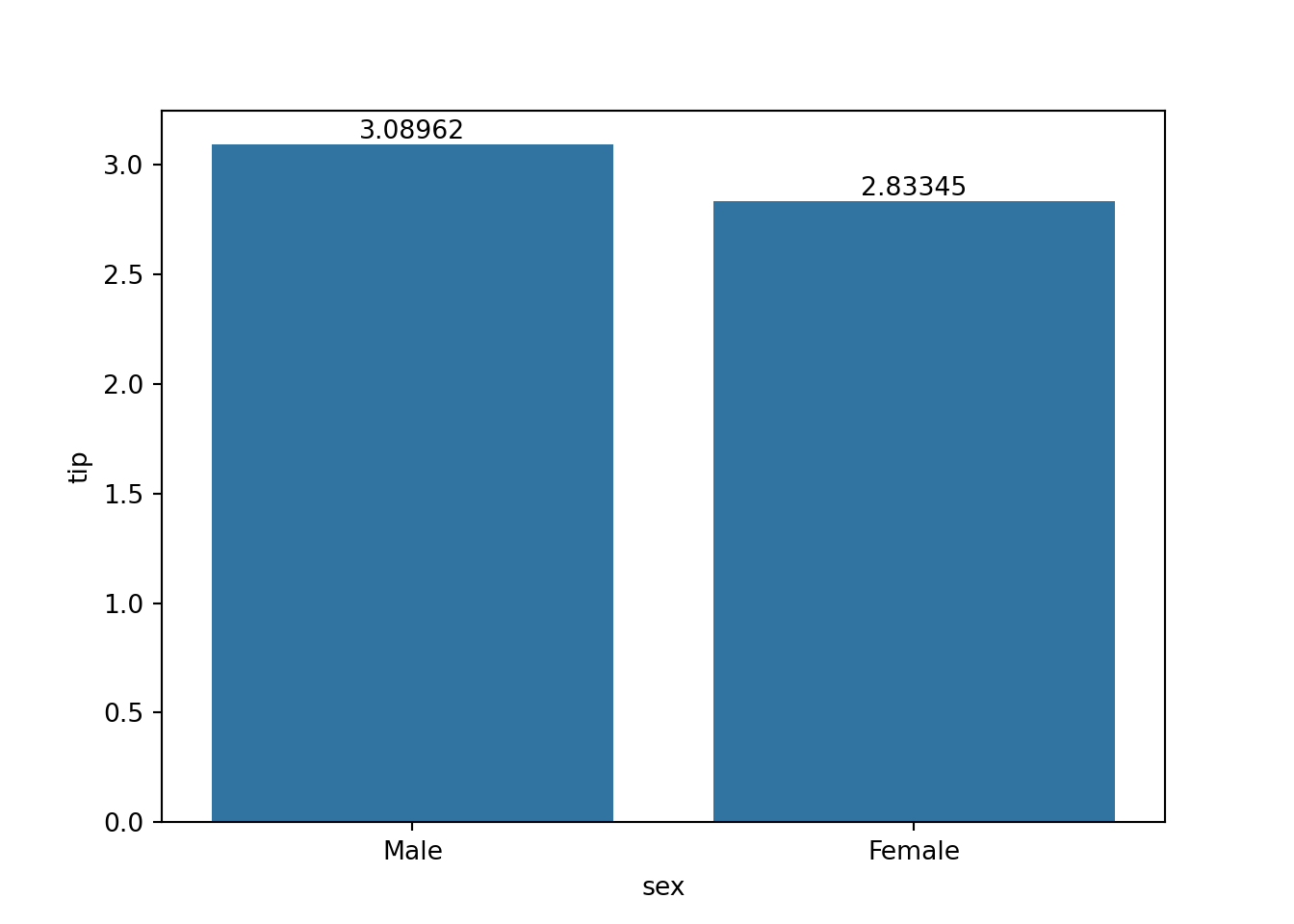
Bar charts can also be plotted horizontally.
ax = sns.barplot(data=tips, y='sex', x='tip', errorbar=None, orient='h')
plt.show()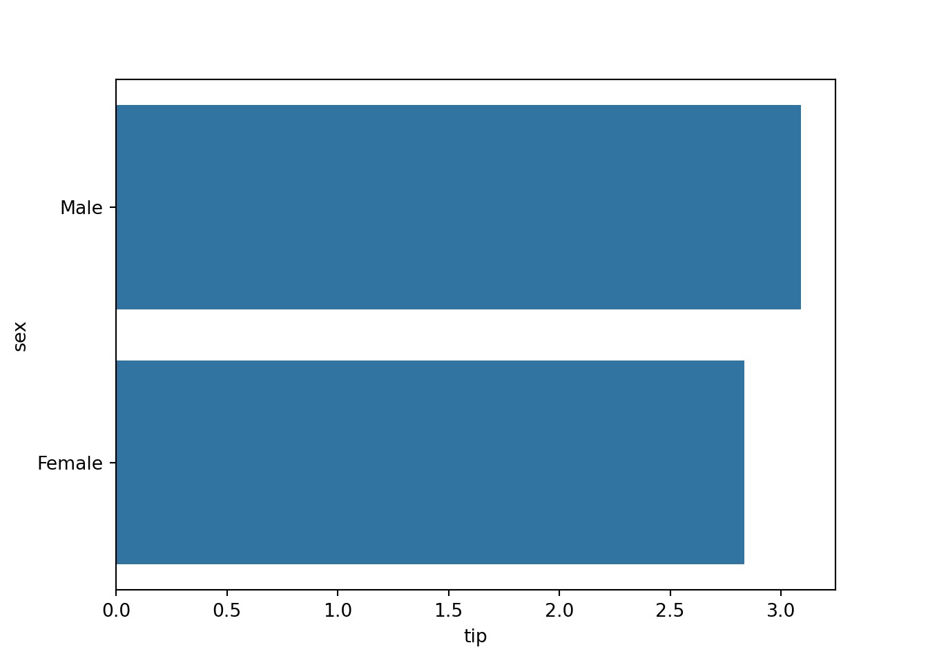
A box plot displays the five-number summary of a set of data: minimum, first quartile, median, third quartile, and maximum.
sns.boxplot(data=tips, x='day', y='tip')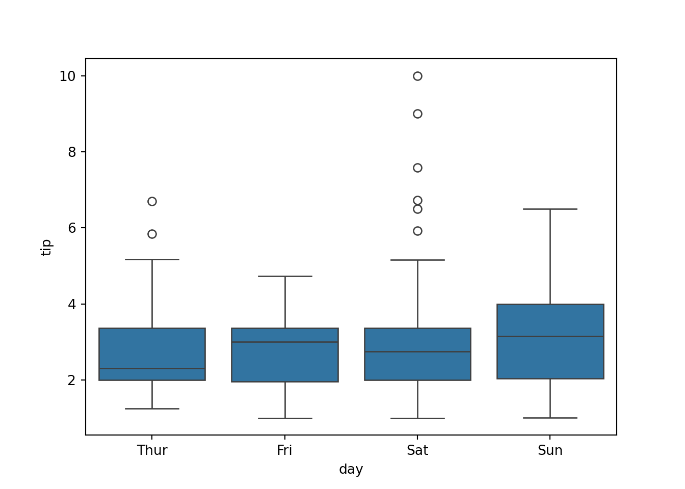
Box plots can be grouped by a categorical variable to compare the distributions.
sns.boxplot(data=tips, x='day', y='tip', hue='sex')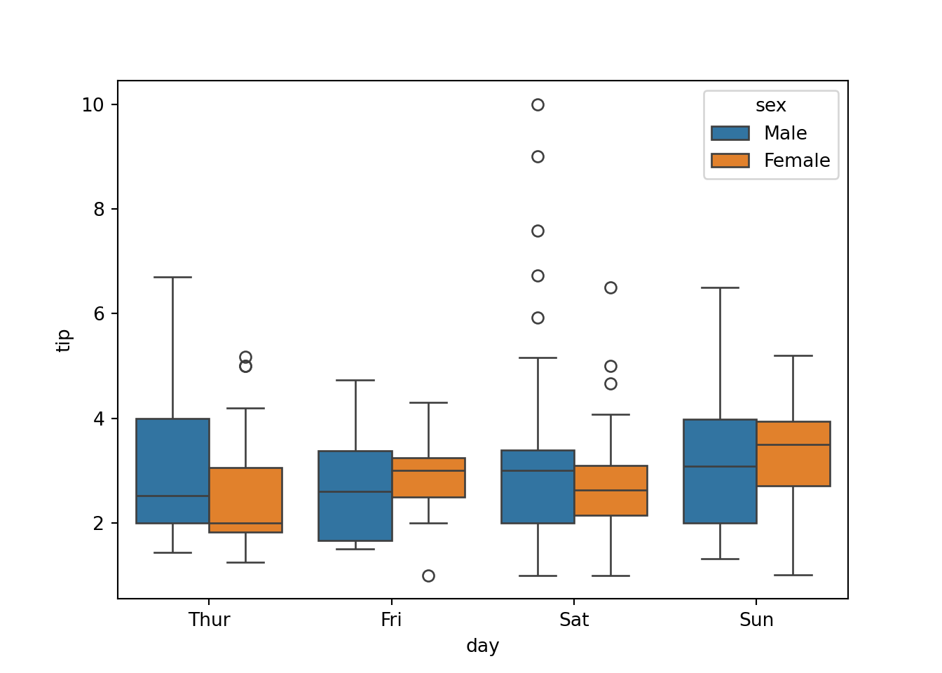
A strip plot is a scatter plot where one of the variables is categorical. It is useful for visualizing the distribution of data points.
sns.stripplot(data=tips, x='day', y='tip')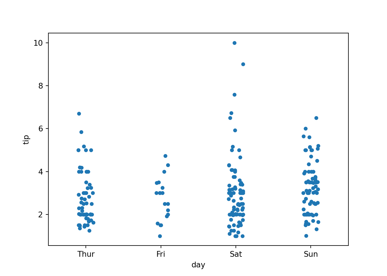
Strip plots can also be grouped by a categorical variable.
sns.stripplot(data=tips, x='day', y='tip', hue='sex', dodge=True)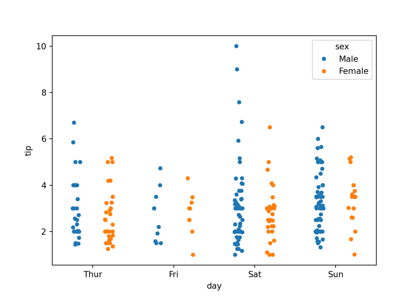
A joint plot shows the relationship between two variables along with their individual distributions.
sns.jointplot(data=tips, x='total_bill', y='tip', kind='reg')<seaborn.axisgrid.JointGrid object at 0x1118ed110>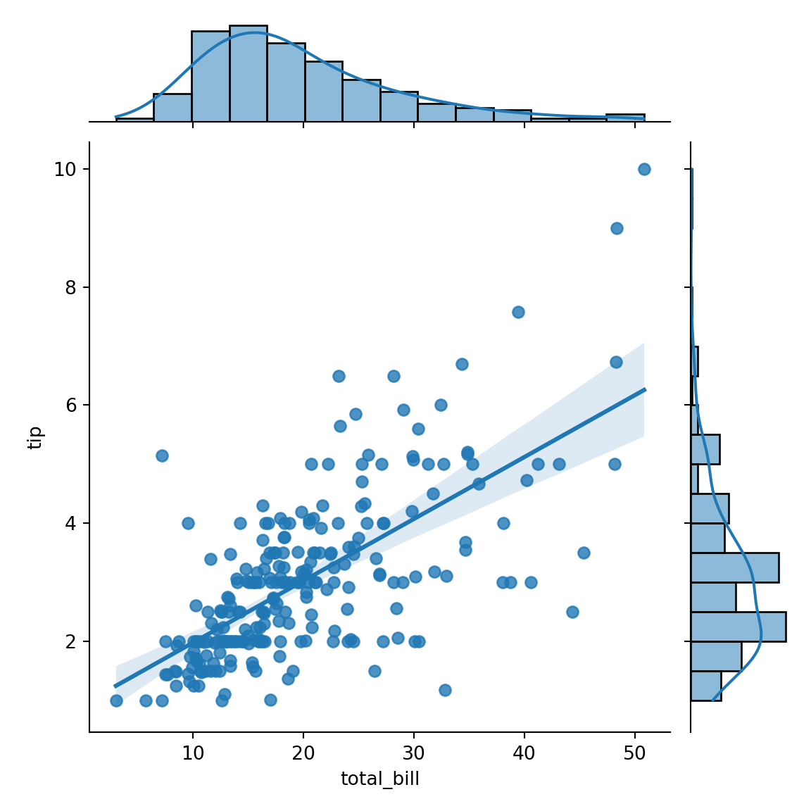
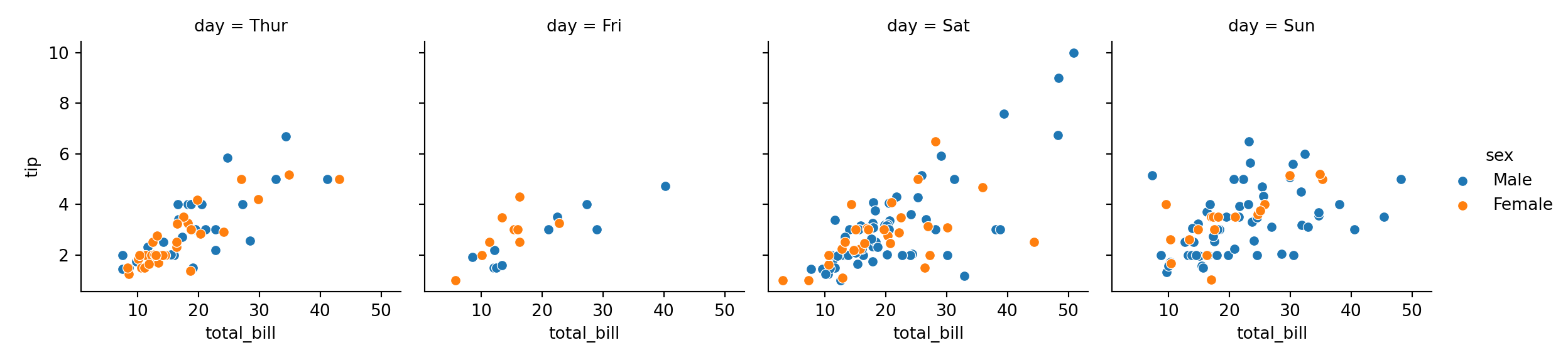
Facet plots allow you to create multiple plots based on the subsets of your data.
g = sns.FacetGrid(data=tips, col="day", hue="sex")
g.map_dataframe(sns.scatterplot, x="total_bill", y="tip")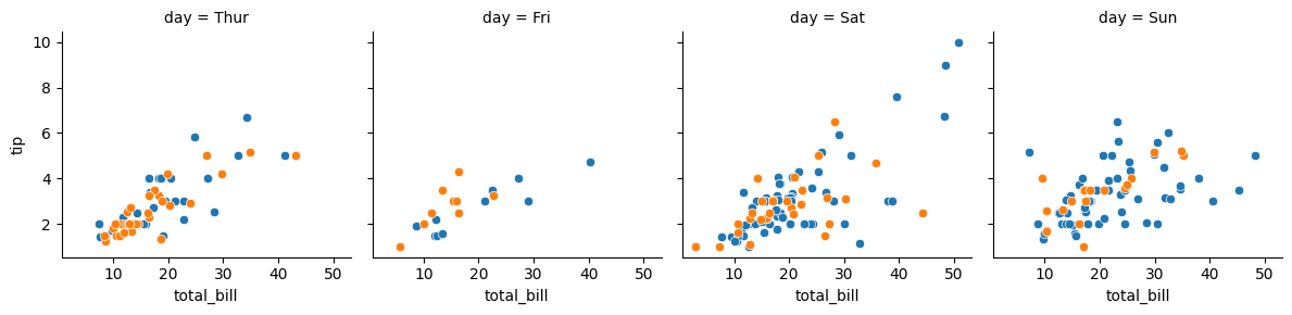
g.add_legend()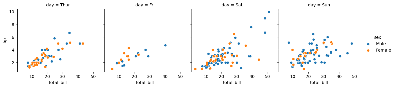
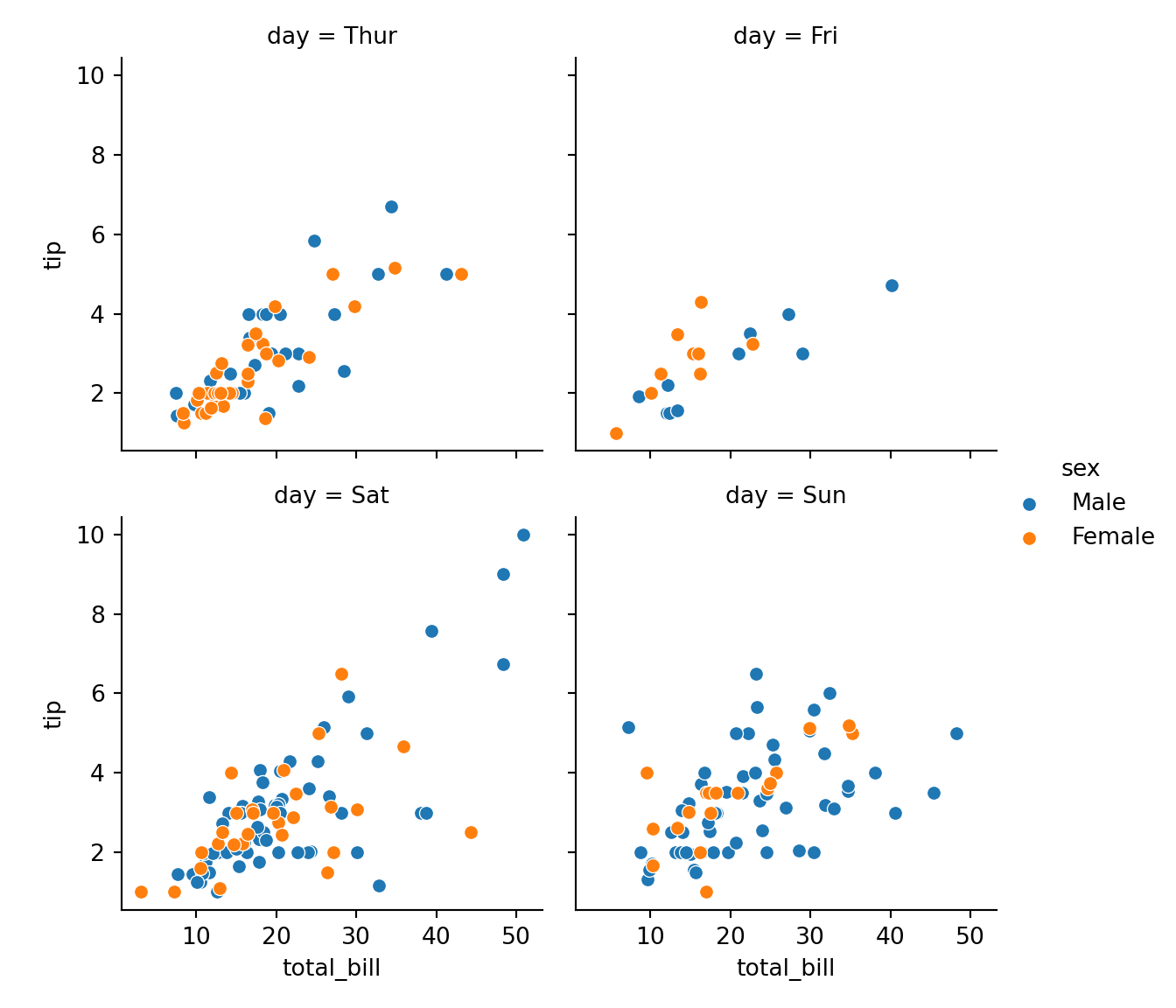
You can wrap the columns of the facet grid to control the layout.
g = sns.FacetGrid(data=tips, col="day", col_wrap=2, hue="sex")
g.map_dataframe(sns.scatterplot, x="total_bill", y="tip")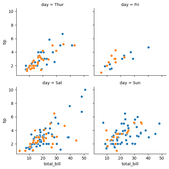
g.add_legend()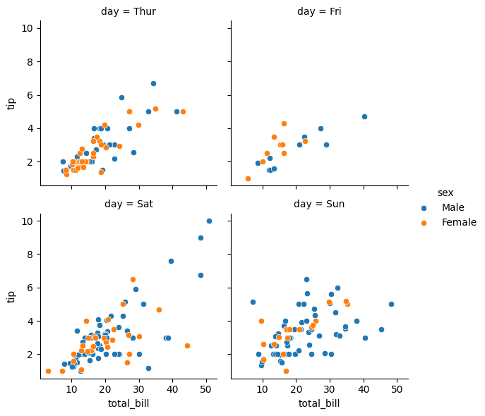
You can create a figure with multiple subplots to display several plots at once.
fig, axes = plt.subplots(1, 2)

sns.boxplot(data=tips, x='day', y='tip', hue='sex', ax=axes[0])
sns.boxplot(data=tips, x='day', y='tip', ax=axes[1])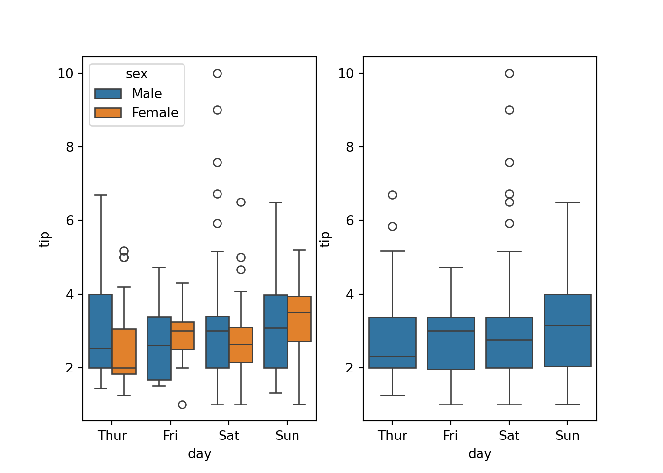
To display Chinese characters correctly in plots on macOS, you need to set the font family to one that supports them.
# Add the following line
plt.rcParams['font.family'] = ['Arial Unicode MS'] # To display Chinese labels correctly
plt.rcParams['axes.unicode_minus'] = False # To display the minus sign correctly
sns.set_style('whitegrid', {'font.sans-serif': ['Arial Unicode MS', 'Arial']})You can add a title to your plot to describe its content.
df = sns.load_dataset("tips")
ax = sns.boxplot(x="day", y="total_bill", data=df)
ax.set_title("Tips Box Plot")
The size of the plot can be adjusted to fit your needs.
plt.clf()
plt.figure(figsize=(10, 6))
ax = sns.boxplot(x="day", y="total_bill", data=df)
ax.set_title("Tips Box Plot")
plt.show()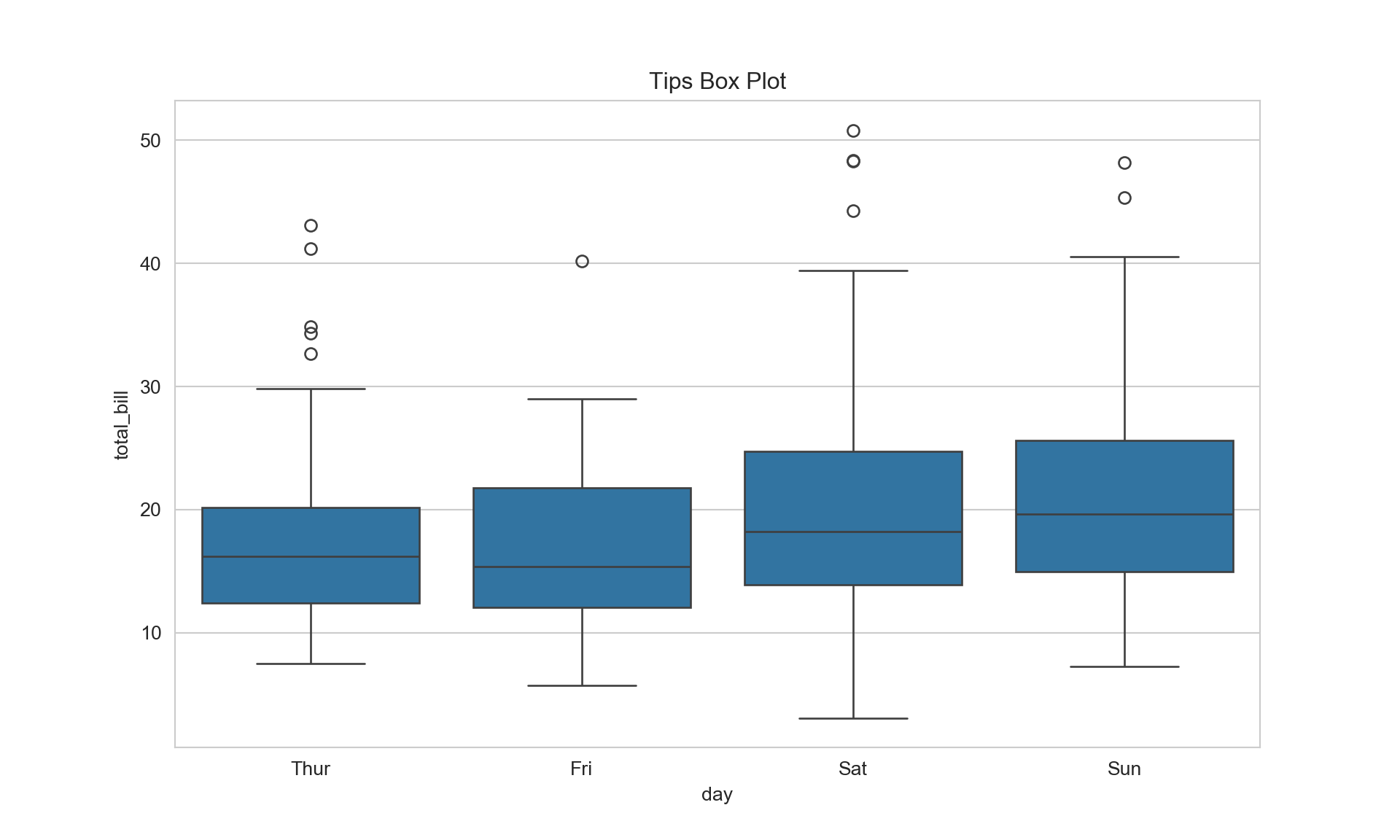

You can customize the labels for the x and y axes.
ax = sns.boxplot(x="day", y="total_bill", data=df)
ax.set_title("Tips Box Plot")
ax.set(xlabel='X-axis Label', ylabel='Y-axis Label')
Seaborn comes with several built-in themes to style your plots.
The “darkgrid” theme is the default and features a gray background with white grid lines.
import seaborn as sns
df = sns.load_dataset("tips")
sns.set_theme()
# Equivalent to:
# sns.set_style("darkgrid")
sns.boxplot(x="day", y="total_bill", data=df)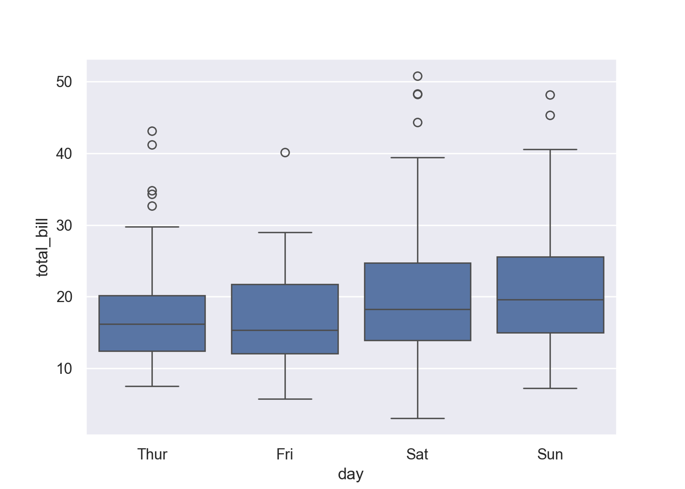
The “whitegrid” theme has a white background with gray grid lines.
import seaborn as sns
df = sns.load_dataset("tips")
sns.set_style("whitegrid")
sns.boxplot(x="day", y="total_bill", data=df)
The “dark” theme is similar to “darkgrid” but without the grid lines.
import seaborn as sns
df = sns.load_dataset("tips")
sns.set_style("dark")
sns.boxplot(x="day", y="total_bill", data=df)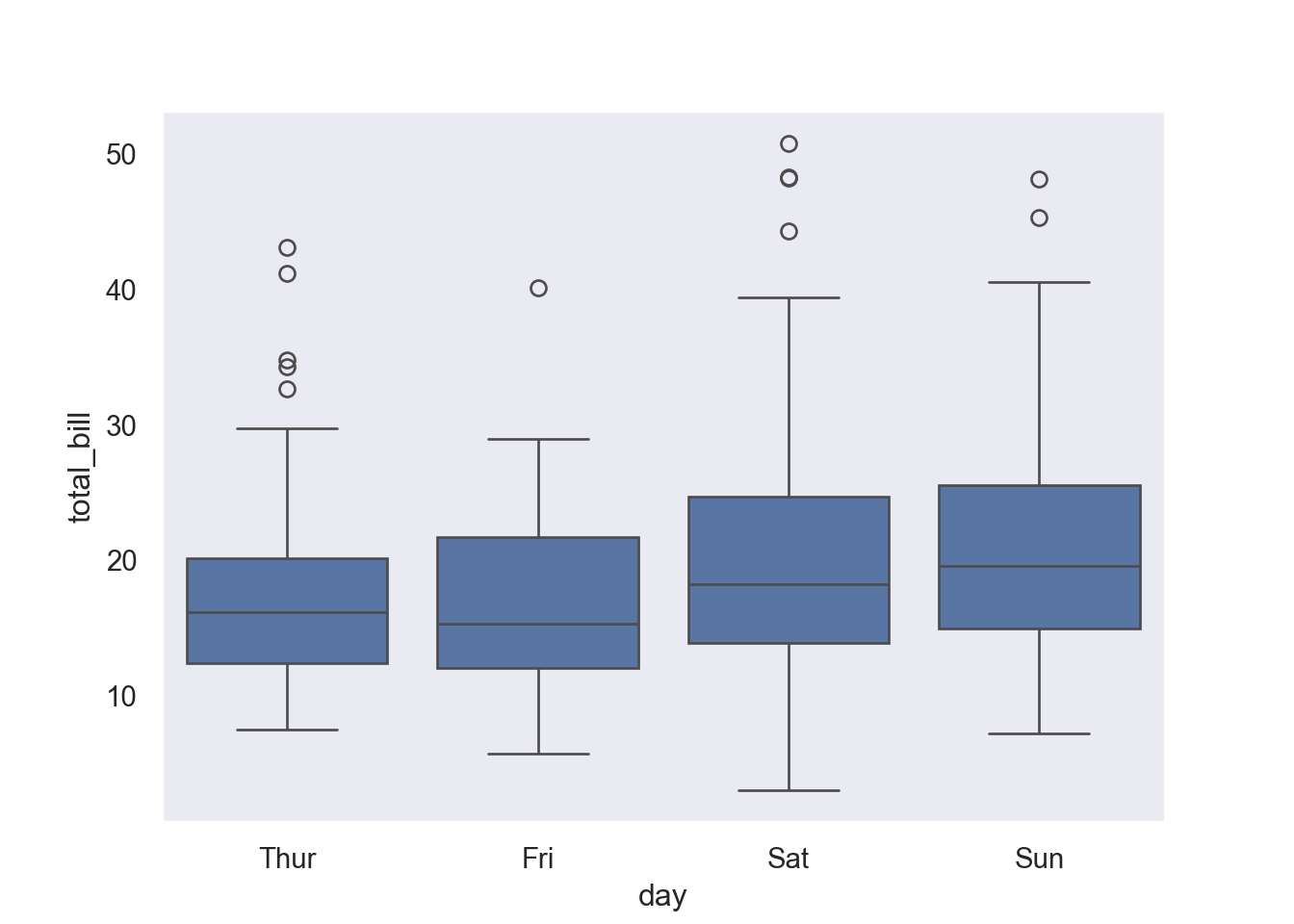
The “white” theme is similar to “whitegrid” but without the grid lines.
import seaborn as sns
df = sns.load_dataset("tips")
sns.set_style("white")
sns.boxplot(x="day", y="total_bill", data=df)
The “ticks” theme is like the “white” theme but adds ticks to the axes.
import seaborn as sns
df = sns.load_dataset("tips")
sns.set_style("ticks")
sns.boxplot(x="day", y="total_bill", data=df)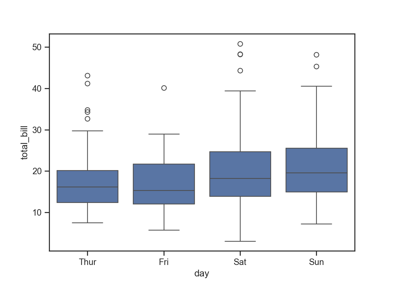
This theme mimics the style of the FiveThirtyEight website.
plt.clf()
plt.style.use('fivethirtyeight')
sns.boxplot(x="day", y="total_bill", data=df)
plt.show()
This theme emulates the popular ggplot2 library in R.
plt.clf()
plt.style.use('ggplot')
sns.boxplot(x="day", y="total_bill", data=df)
plt.show()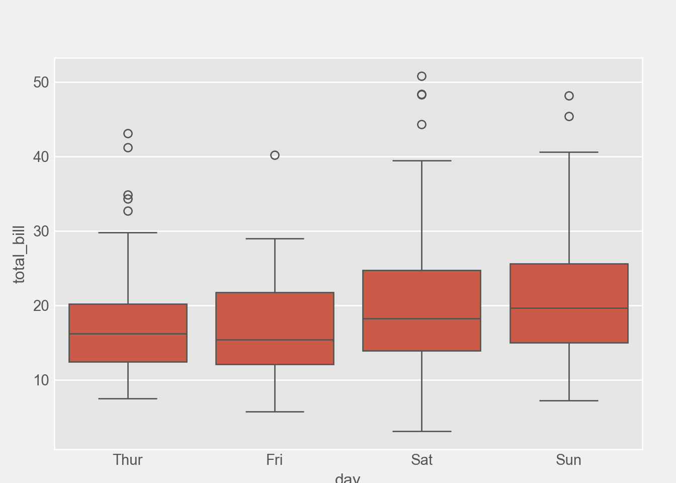
This theme uses a color palette that is friendly to colorblind viewers.
plt.clf()
plt.style.use('tableau-colorblind10')
sns.boxplot(x="day", y="total_bill", data=df)
plt.show()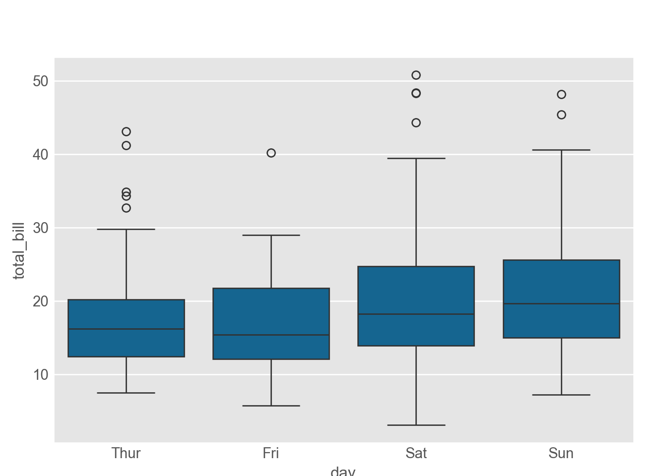
This theme uses a dark background for the plots.
plt.clf()
plt.style.use('dark_background')
sns.boxplot(x="day", y="total_bill", data=df)
plt.show()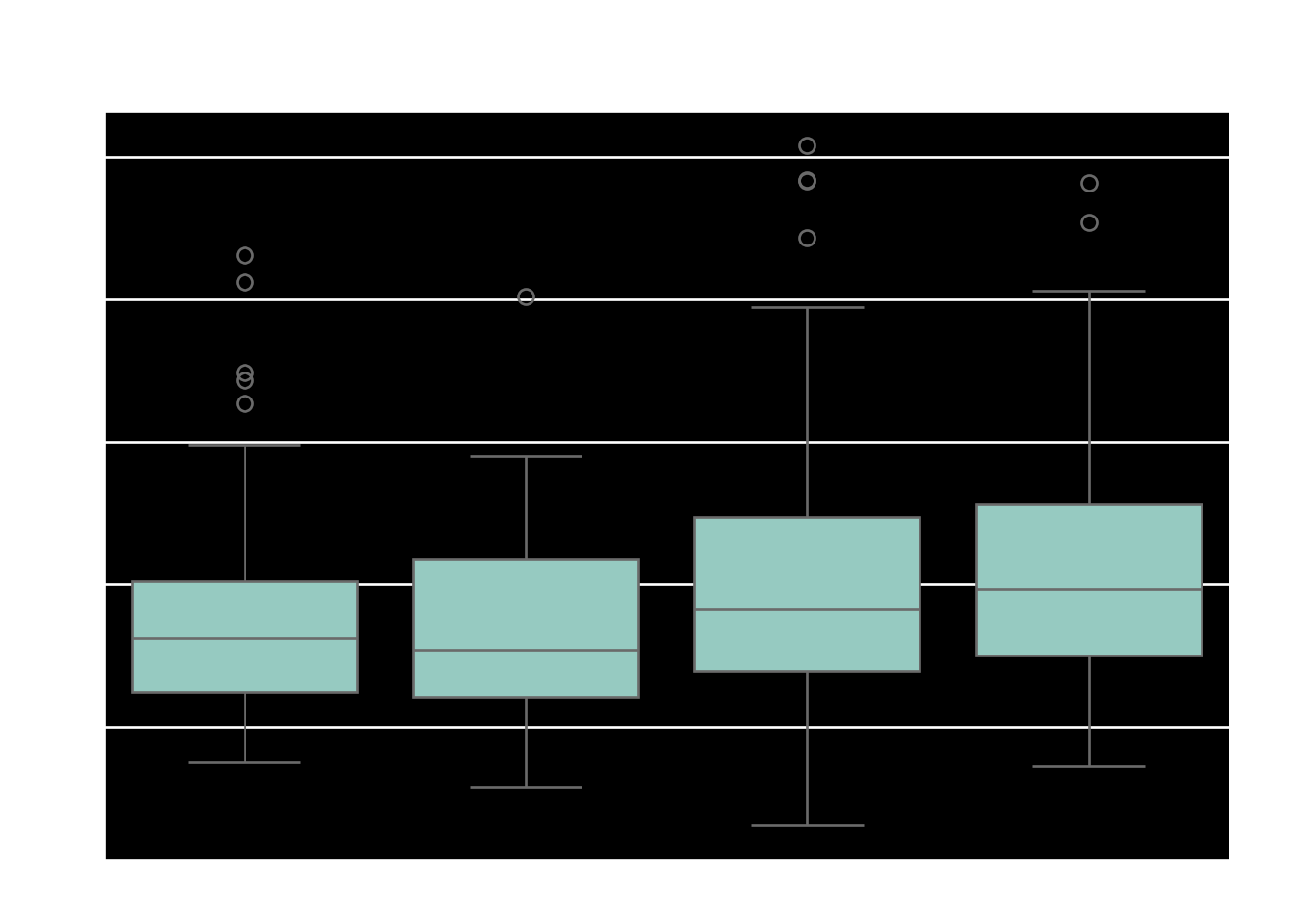
You can save your plot to a file in various formats.
import seaborn as sns
df = sns.load_dataset("tips")
plt.clf()
plt.style.use('default')
sns.boxplot(x="day", y="total_bill", data=df)
plt.savefig("output.png", dpi=100, bbox_inches="tight")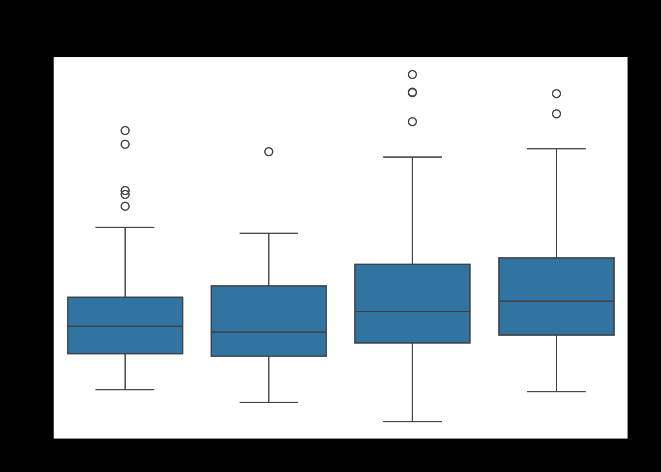
You can create animated plots to show changes over time or another variable.
from celluloid import Camerafrom celluloid import Camera
from matplotlib import pyplot as plt
fig = plt.figure()
camera = Camera(fig)
a = sns.lineplot(data=dowjones4, x='Date', y='Price', hue='type')
hands, labs = a.get_legend_handles_labels()
new_data = dowjones4.sample(50, random_state=42)
new_data = new_data.sort_values(by=['Date'], ascending=True)
for i in new_data["Date"]:
data = dowjones4.query('Date <= @i')
sns.lineplot(data=data, x='Date', y='Price', hue='type')
plt.legend(handles=hands, labels=labs)
camera.snap()
animation = camera.animate()from IPython.display import HTML
HTML(animation.to_html5_video())